One of the hardest Spark concepts to grasp is that of a Spark shuffle, but it is also usually the biggest performance killer. Conversely, a good understanding of shuffles can help you optimize your biggest bottlenecks. This post focuses on how to reason about shuffles and their performance impact.

Partitions

A partition is a logical chunk of a large dataset. Since Spark is a distributed engine, it breaks data into these chunks so different nodes (Executors/Cores) can work on them in parallel. By default, Spark targets partitions of around 128MB when reading files, controlled by spark.sql.files.maxPartitionBytes.

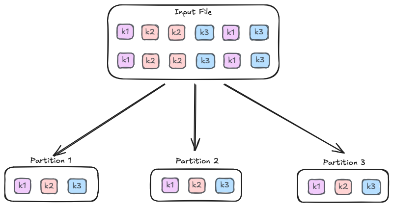
For instance, when reading a large file of 1GB, Spark may split it into 7–8 partitions of ~128MB each. Conversely, when reading thousands of small files, Spark may choose to “coalesce” them into bigger partitions until it hits the target.

The key points to remember are:

• A partition is the logical unit of data processing.
• Each partition corresponds to one task in the Spark UI, which is why partition counts directly translate to task counts.
• All data within a partition is processed by a single task on a single executor at any given time.

Wide vs. Narrow Transformations

When writing Spark code, you’ll typically encounter two kinds of operations:

Narrow Transformations (Fast)

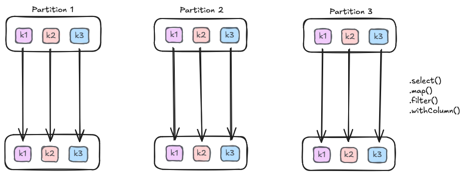
In a Narrow Transformation, each input partition contributes to exactly one output partition, meaning data stays on the same machine. Examples include map(), filter(), withColumn(), and select(). These operations are fast because the data never has to leave the executor. The operation doesn’t depend on other rows in the dataset; for example, Spark can independently map a record to a new value in memory.

Wide Transformations (Slow)

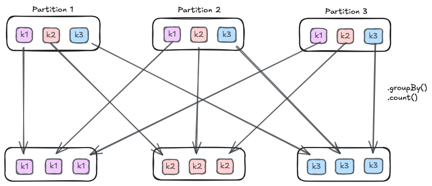
Wide Transformations are those where the output may depend on multiple input partitions. For instance, when performing aggregations by a key, Spark needs to know what records exist for a given key in all the partitions of the dataset. As a result, data from one partition will need to move to another partition either between different cores on the same JVM, or in the worst case, over the network between executors. Wide transformations introduce a stage boundary, meaning Spark must finish one set of tasks before starting the next.

The Cost: Why Shuffle Kills Performance

A shuffle is essentially how Spark performs a wide transformation. While necessary, a shuffle comes with a few downsides:

I/O and Serialization Overhead

During a shuffle, Spark cannot simply move data in memory. To efficiently move data between executors, it must first serialize it and store it on local disk (the Shuffle Write). Similarly, the receiving executor must then deserialize the data before it can be processed (the Shuffle Read). Both operations are CPU intensive and consume network bandwidth. This combination of disk I/O and network transfer is orders of magnitude slower than RAM-based processing.

Skewed Data

While shuffles are slow by themselves, they become especially problematic when data is highly skewed. In real-world datasets, data is often dominated by a single key — for example, a handful of users responsible for the majority of activity.

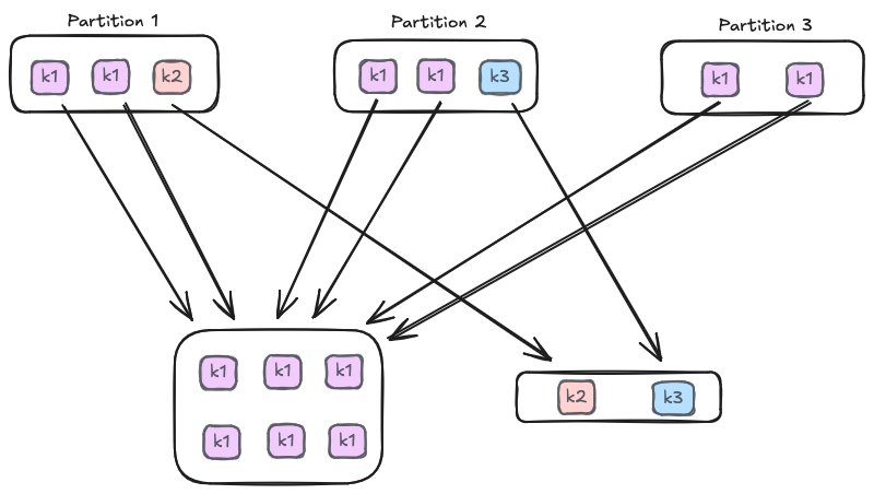
In these cases, Spark tries to pull all data for that skewed entity into a single partition, creating a bottleneck where one executor works on a massive task while others sit idle. This single “straggler” task determines the execution time for the entire job. In Spark UI, this typically shows up as one task in a shuffle stage running far longer than the rest, often with much higher shuffle read bytes.

Importantly, increasing the number of executors does not fix skew — because the skewed partition is still processed by a single task.

Memory Contention

As noted in the previous post, Spark divides executor memory into two main pools: Storage (for cached data) and Execution (for shuffles and joins), which can borrow from each other under pressure. If a shuffle requires more memory than is available in the Execution pool, it will start “evicting” cached data from the Storage pool. If it still needs more, Spark will “spill” the shuffle data to disk, which slows down the operation significantly because disk access is much slower than RAM.

What can you change?

Shuffles are inevitable in data processing. Computing aggregates and joins are all necessary operations and cannot be completely avoided. However, a few simple strategies mitigate the impact:

Reduce the data being shuffled

Shuffling is expensive because of the volume of data moving across the network. Always filter() rows and select() only the columns you truly need before a wide transformation. This minimizes the payload written to disk and sent over the wire. Reducing row width is often just as important as reducing row count.

Broadcast joins

If you are joining a large table with a small one, use a broadcast() hint. This sends a copy of the small table to every executor, allowing the join to happen locally within each partition. This effectively turns a wide join into a narrow one and skips the shuffle entirely. Broadcast joins work best when the broadcasted table comfortably fits in executor memory.

Tune Shuffle Partitions

The configuration spark.sql.shuffle.partitions defaults to 200. This is rarely the right number. If your data is tiny, 200 tasks create massive scheduling overhead; if your data is massive, 200 tasks may create partitions so large they cause OOM errors. Tune this number so that your post-shuffle partitions are roughly 128MB to 200MB each.

Apply Salting (Advanced)

For severe data skew, you can implement “Salting”. This involves adding a random integer (the “salt”) to your join or grouping key. This forces Spark to distribute a single “hot” key across multiple partitions rather than cramming it into one. While this requires an extra step to aggregate the results back together, it is often the only way to bypass a “straggler” task.

Final Thoughts

Shuffles aren’t bad — but they are expensive. Understanding when they happen, why they hurt, and how to mitigate them is the key to writing performant Spark jobs.